Random Forest

Problem statement

Before reaching for deep sequence models on the plasma state classification problem, I needed a strong, interpretable baseline. Random Forest fit the bill: an ensemble of decision trees is robust to noisy sensors, tolerant of missing values (a common fact of life in tokamak diagnostics), and gives feature importances that can be sanity-checked against plasma physics intuition. The question I was trying to answer in this thread was whether a classical, no-frills model could reliably separate the four operational states of a tokamak plasma (Suppressed, Mitigated, ELMing, Dithering) from standard diagnostic features, and if so, which features and which evaluation protocol actually made those numbers honest.

My role and contributions

This was the first end-to-end ML model I owned on the project. I:

• Curated and hand-labeled the dataset on the DIII-D iris cluster using OMFIT and reviewplus, growing it from 36 shots to 88 shots (~200,000 one-millisecond points) over successive run campaigns.
• Built the full scikit-learn Random Forest pipeline: feature extraction from the DIII-D MDSplus diagnostic tree, stratified train/validation/test splits, and two parallel evaluation protocols (point-wise and shot-wise) so we could quantify how much accuracy came from real signal versus shot memorization.
• Ran forward feature selection across the available diagnostics to land on a compact, physics-relevant feature set.
• Designed a sequential hyperparameter search across ~600 configurations so each tuning step was traceable and defensible to physics collaborators.
• Used the trained model to run causal use-case sweeps: fix every feature at its median and vary one at a time to extract RF-predicted suppression probability as a function of electron density, coil currents, and other operator-controllable knobs.

Dataset and labels

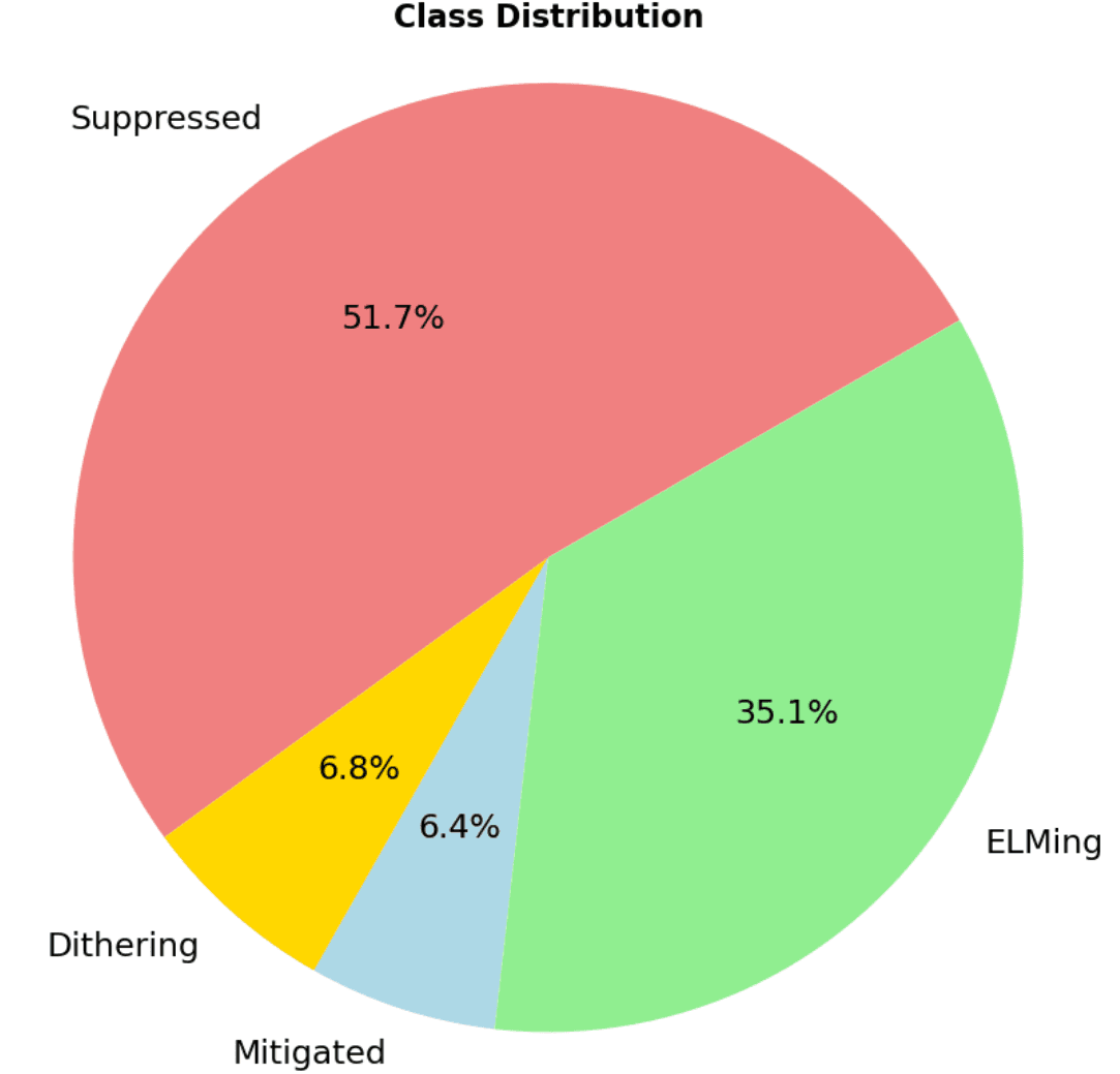
The dataset is DIII-D H-mode discharges from 2017 to 2023 that actually applied RMPs, sampled at 1 ms. States were hand-labeled off the FS04 filterscope Dα signal plus supporting diagnostics. The class balance is heavily skewed, which ended up being an important shape of the problem:

Feature selection

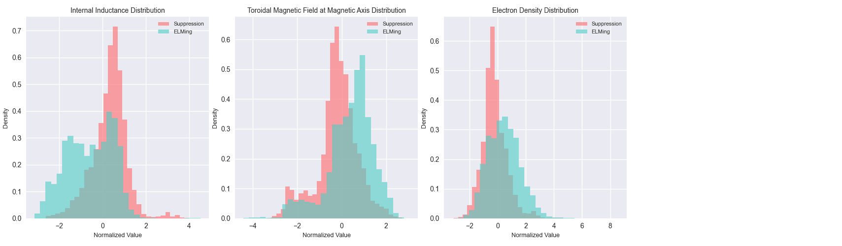
I ran forward selection: start with no features, add the single feature that most improves held-out accuracy, fix it, and repeat. The final compact set included the four RMP coil current amplitudes (iln3iamp, iln2iamp, iun2iamp, iun3iamp), normalized plasma pressure βN, pedestal separation ΔR_sep, plasma and pedestal electron density, internal inductance ℓᵢ, upper triangularity, and the FS04 Dα signal.

The headline visual test of whether the most important single features can separate the states is below. They can, but not cleanly:

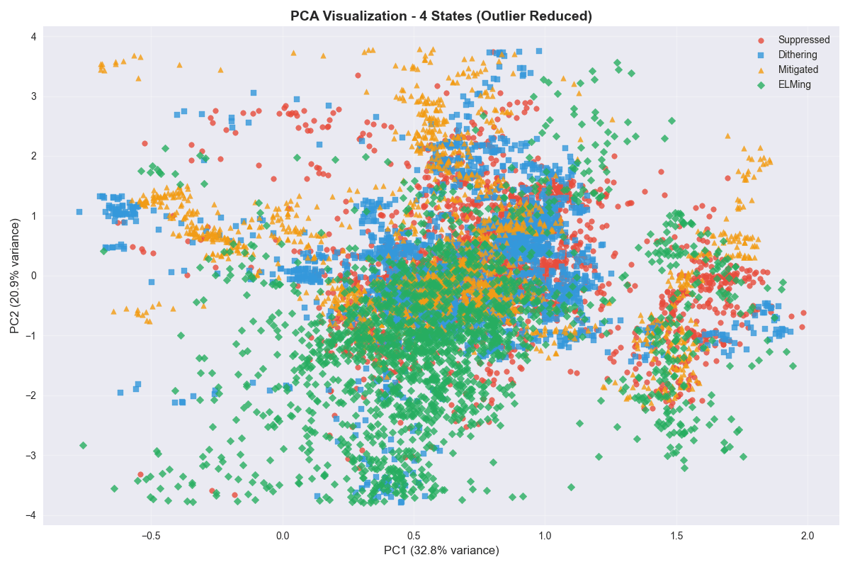
Projecting into the first two principal components tells the same story:

Hyperparameter search

I used a sequential one-axis-at-a-time search rather than a full grid or random search, for two reasons. First, with roughly 600 candidate configurations the grid was small enough to scan deliberately, and second, collaborators from the physics side could follow a step-by-step narrative ("we set n_estimators to 400 because accuracy plateaued there, then held that fixed while we swept max_depth, and so on") far more easily than they could interpret the output of a random search.

Tuned axes included n_estimators, max_depth, min_samples_split, min_samples_leaf, max_features, class_weight, and the bootstrap sample rate, with stratified k-fold cross-validation on every sweep so that the rare Mitigated and Dithering classes were never starved out of the validation fold.

Evaluation protocols

This is where the project taught me the most. The same Random Forest, on the same dataset, gives wildly different accuracy numbers depending on how you split.

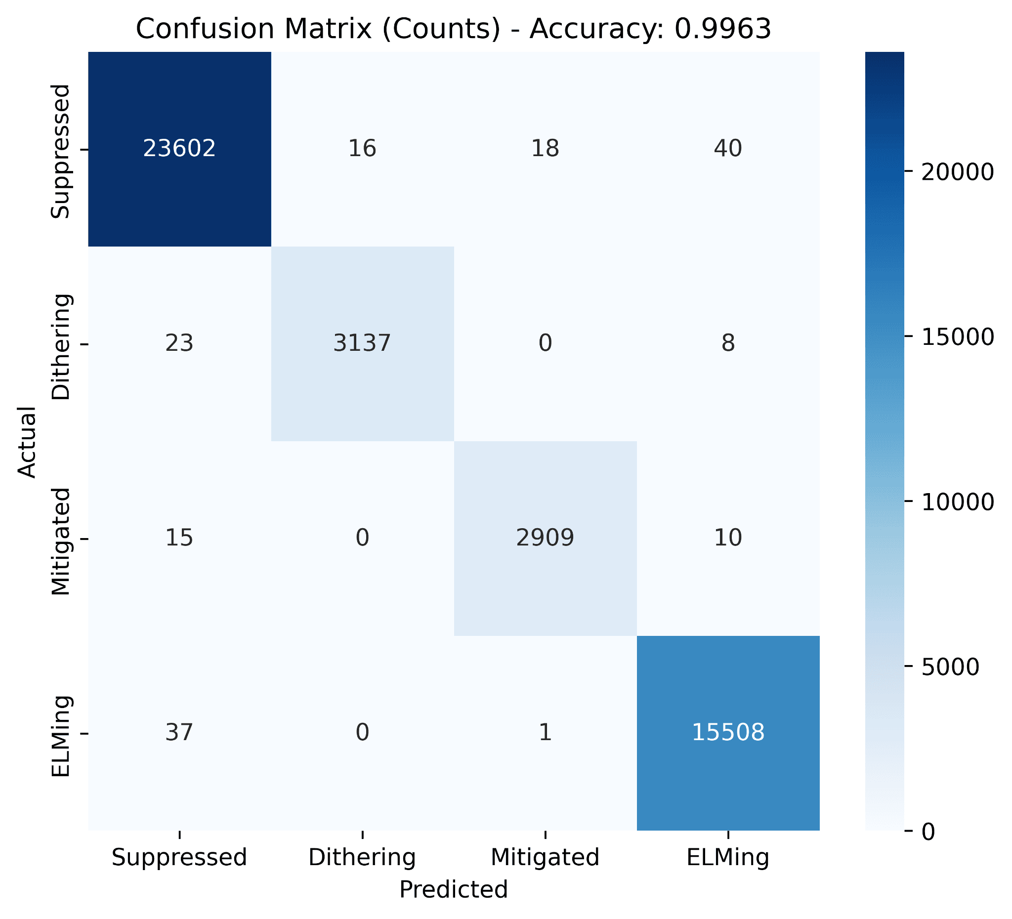
Point-wise split (random across all ms samples from all 88 shots) looks like this:

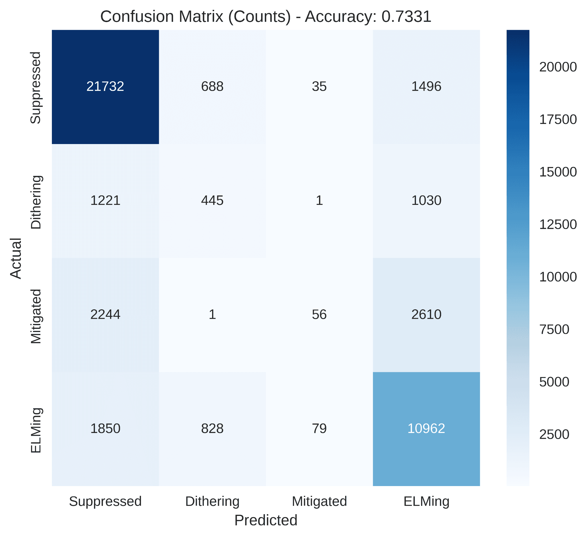
Shot-wise split (hold out whole shots the model has never seen) tells the real story:

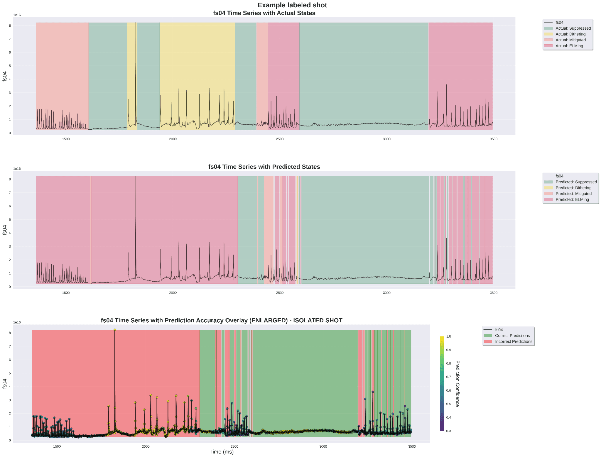
To pressure-test qualitatively on a shot that was completely held out, I overlaid the Random Forest predictions on the FS04 time series and the actual labels:

Use-case sweeps

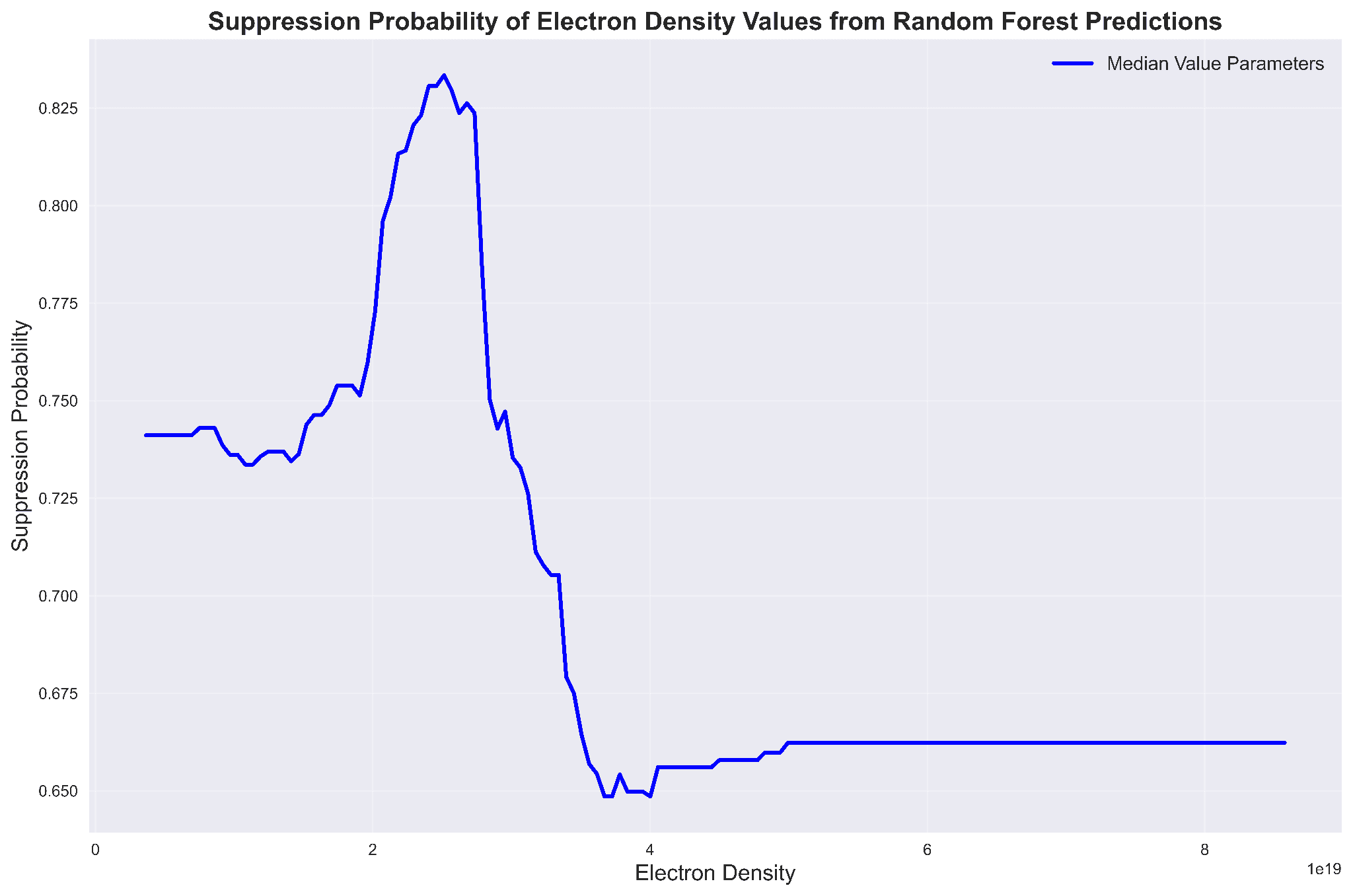
Once the Random Forest was trained, I used it as a cheap surrogate for asking "if an operator changed one knob and held everything else at its typical (median) value, how does the predicted probability of being suppressed respond?". These sweeps are the most physically actionable thing a classical model like this can produce.

Electron density sweep:

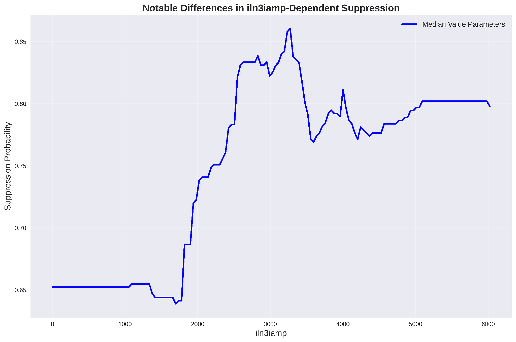
Internal lower n=3 RMP coil current sweep:

Results summary

• Random Forest exploration across roughly 600 hyperparameter configurations under stratified cross-validation.
• 99.6% point-wise accuracy and 71.5% to 73.3% shot-wise accuracy on the four-state task on the 88-shot, ~200K-point dataset, depending on the specific held-out shot set.
• Precision and recall comfortably above 0.85 on Suppressed, Mitigated, and ELMing in the point-wise regime; Dithering is harder (~0.73 recall) because by definition it is a transient state with very few ms of training signal per shot.
• Feature-distribution and use-case findings line up with pedestal physics: suppression concentrates at peaked current profiles (higher ℓᵢ) and moderate electron density (~3.7×10¹³ on the edge, ~2.5×10¹⁹ m⁻³ for core ne sweep), and there is a clean optimum in the n=3 coil current amplitude.
• The point-wise vs shot-wise accuracy gap was the single most useful methodology outcome of the whole thread. It set the evaluation standard that every later model (CNN-BiLSTM, TCN, LSTM forecaster) had to be judged against.

Stack notes

scikit-learn, Python, NumPy, pandas, Matplotlib, stratified k-fold cross-validation, forward feature selection, OMFIT and reviewplus on the DIII-D iris compute cluster for pulling and hand-labeling experimental data, in collaboration with Columbia Fusion Research Center.